1.2 What is a Neural Network?

An Example

Housing Price Prediction

Size (x) → (a circle) (neuron) → Price (y^)

ReLU function (rectified linear unit): “rectified” here means taking the maximum of zero and the input.

ReLU(z)=max(0,z)

This is a small neural network.

Adding Other Features

Like bedrooms, zip code (postal code, maybe as a feature that tells you about walkability), and wealth.

Then you have a neural network with 4 inputs, including size.

These circles in the hidden layer are called hidden units in a neural network.

2.1 Binary Classification & Notation Convention

y: 1 (cat) vs. 0 (non-cat).

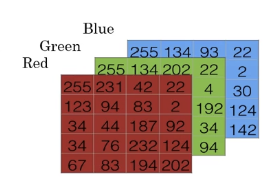
How your computer stores an image:

RGB image stored as three separate matrices

It stores 3 separate matrices: red, green, and blue.

For a 64×64 RGB image, flatten these matrices into an input feature vector x∈Rnx, where

nx=64×64×3=12,288.

A single training example is represented by a pair (x,y), where x is an nx-dimensional vector and y, the label, is either 0 or 1.

Your training set will comprise m training examples:

(x(1),y(1)), (x(2),y(2)), …, (x(m),y(m)).

m=mtrain is the number of training examples, while mtest is the number of test examples. The superscript (i) indexes the example.

Stack the training examples as columns:
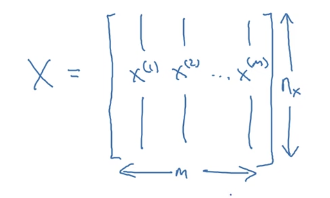
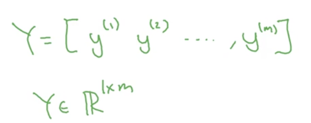
X=[x(1)x(2)⋯x(m)]∈Rnx×m,Y=[y(1)y(2)⋯y(m)]∈R1×m.

Training examples arranged as columns of X

Labels arranged as a row vector Y

2.2 Logistic Regression

z=wTx+b,y^=a=σ(z)=11+e−z.

Here, w∈Rnx, b∈R, and y^ estimates P(y=1∣x).

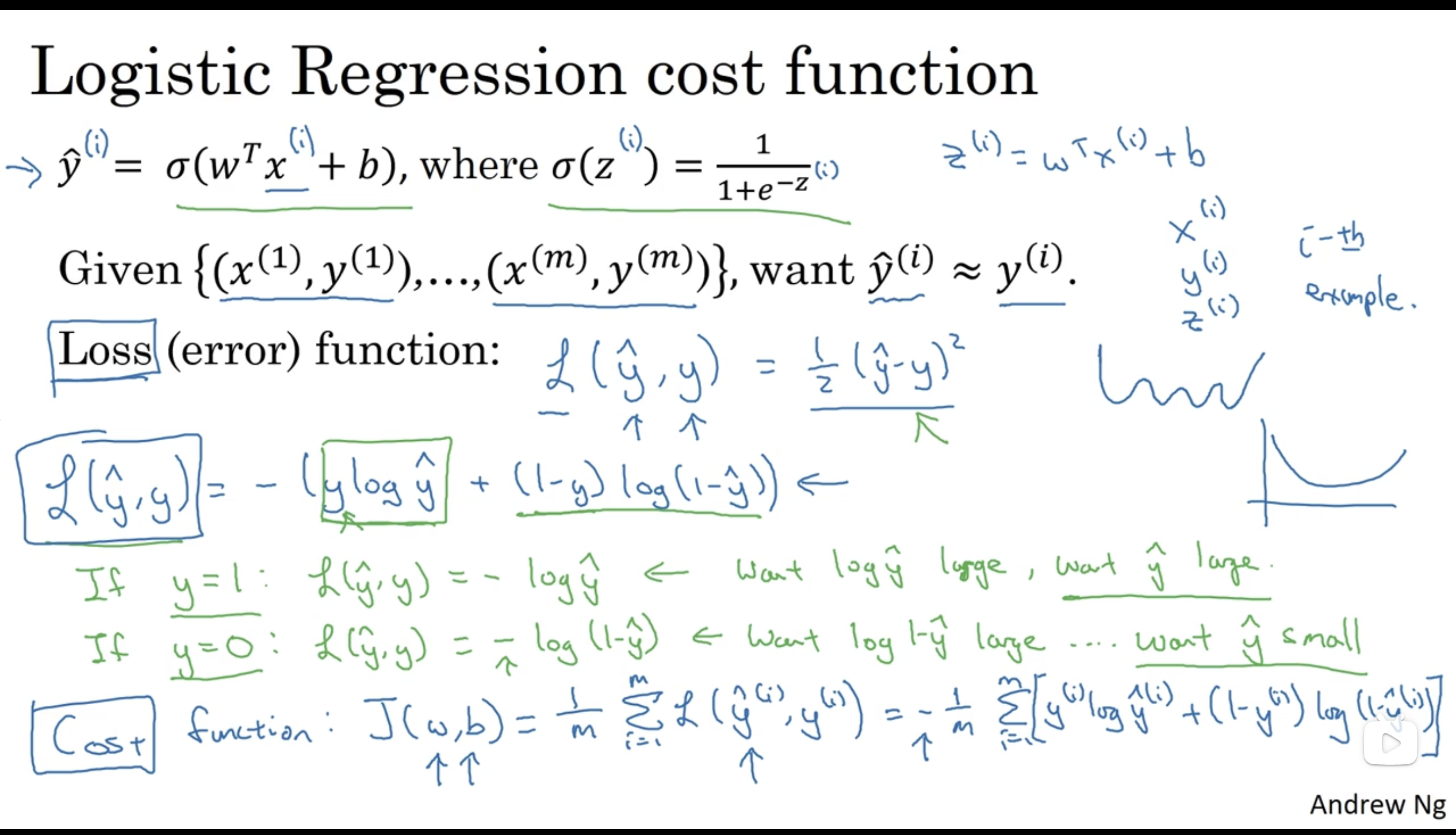
2.3 Logistic Regression: Loss Function

Loss is for a single example; cost is the average loss over the training set.

L(y^,y)=−[ylog⁡y^+(1−y)log⁡(1−y^)].
  • If y=1: L=−log⁡y^; we want y^ large.
  • If y=0: L=−log⁡(1−y^); we want y^ small.
J(w,b)=1m∑i=1mL(y^(i),y(i)).

Logistic regression, loss function, and cost function

2.4 Gradient Descent

Repeat the updates to minimize J(w,b):
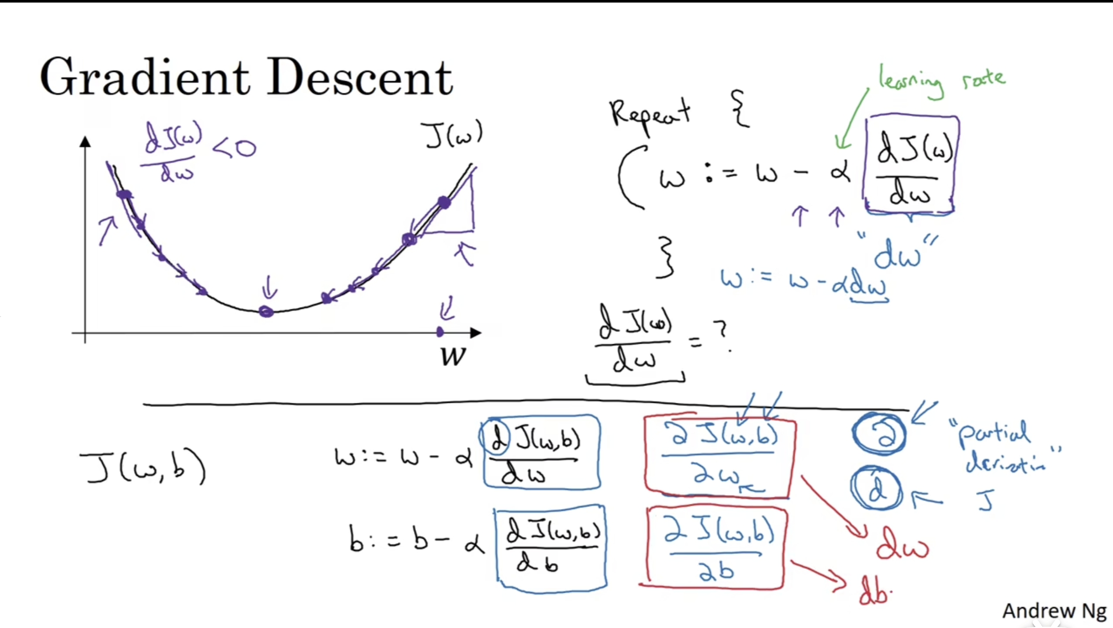
w←w−α∇wJ(w,b),b←b−α∂J(w,b)∂b.

α is the learning rate. Compute both gradients using the current parameters before updating them.

Gradient descent and parameter updates

2.9 Gradient Descent in Logistic Regression

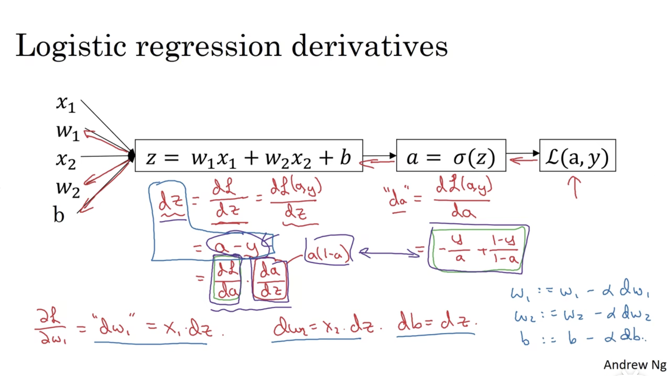
For a single example, with a=σ(z):

dz=∂L∂z=a−y,dwj=∂L∂wj=xjdz,db=∂L∂b=dz.

Here, dz, dwj, and db are shorthand for derivatives.

Logistic regression computation graph and derivatives

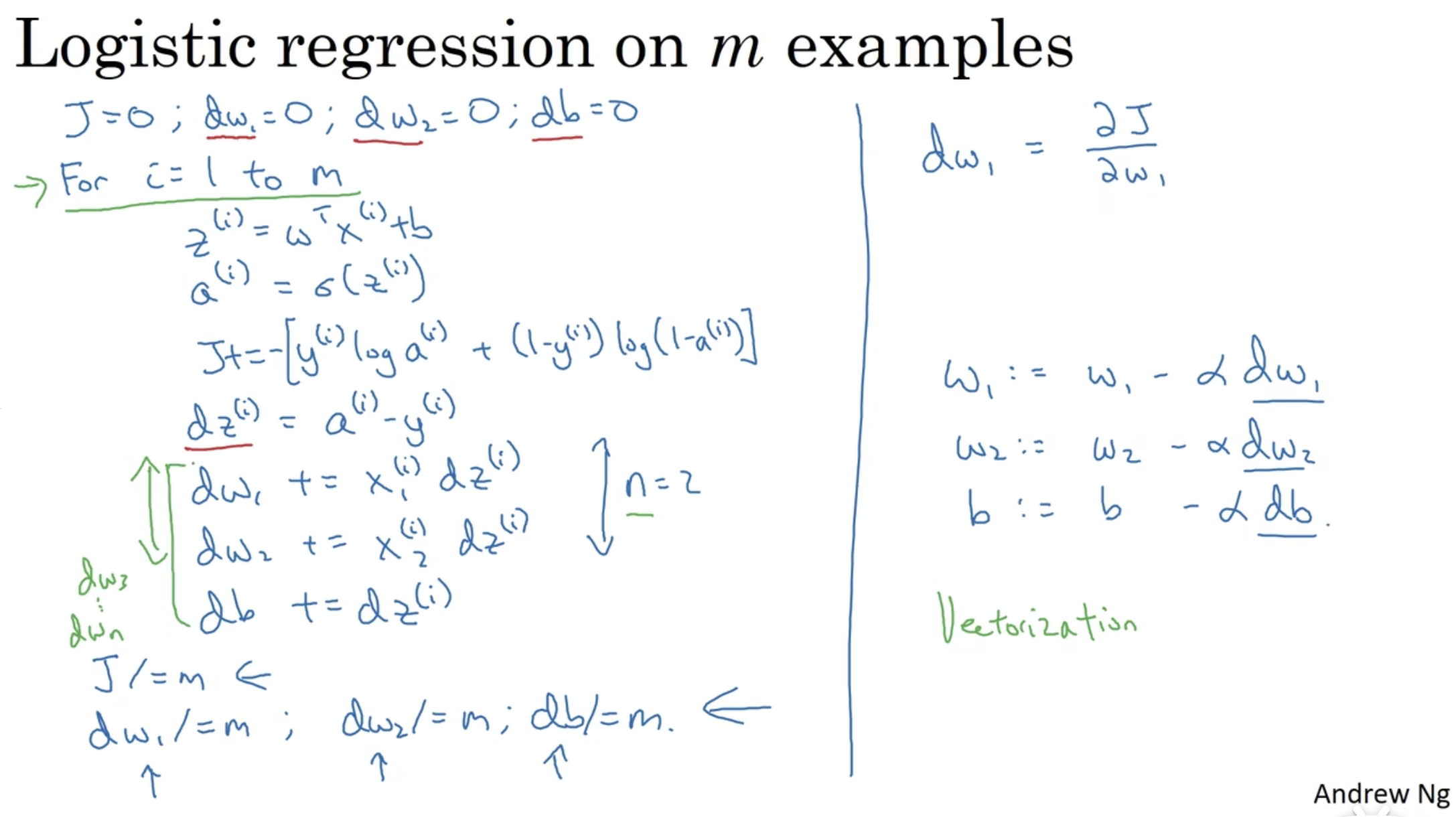
2.10 Logistic Regression on m Examples

Average the gradients over all m examples:

dwj=∂J∂wj=1m∑i=1mxj(i)(a(i)−y(i)),db=∂J∂b=1m∑i=1m(a(i)−y(i)).

Then update wj←wj−αdwj and b←b−αdb.

Logistic regression gradient descent over m training examples

2.11 Vectorization

What Is Vectorization?

In z=wTx+b, w and x are both nx-dimensional column vectors.

Maybe they're very large vectors if you have a lot of features. Using a for loop over j=1,…,nx to calculate dw1,dw2,…,dwnx can take a lot of time. Vectorization uses array operations instead of explicit loops.

A non-vectorized example for calculating z:
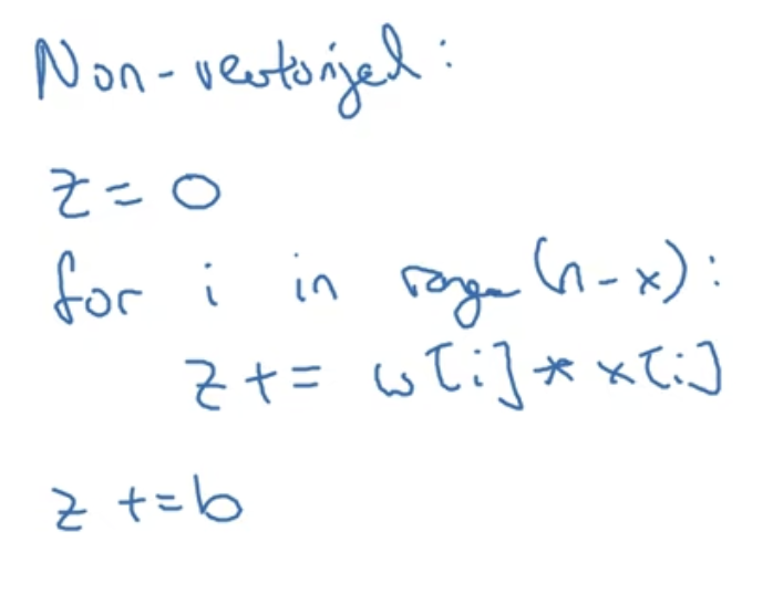
Non-vectorized calculation of z using a for loop

Instead, use (with w and x stored as one-dimensional NumPy arrays):

z = np.dot(w, x) + b

This means z=wTx+b, and it's usually much faster. For explicit column arrays with shape (n_x, 1), use w.T @ x + b.